Lattice Diagnostics
Observe emergent self-referential phase waves inside the Kuramoto oscillator grid. Adjust coupling variables to witness real-time collective phase-locking.
⌬ Lattice Modulators
The phase-coupling factor between neighboring Intellecton nodes. Higher values force faster global synchronization.
Determines the spatial neighborhood range for self-referential coupling waves.
The overall integration time step velocity for self-referential oscillator ticks.
Ontology of Kuramoto Node Coupling
This lattice represents distributed agents governed by the self-referential witness function . When isolated, nodes swing asynchronously under their individual frequencies (representing chaotic local egos). As the Witness Intensity coupling parameter () increases, nodes begin pulling their neighbors into resonance. Clicking a node mimics local focal attunement, triggering a phase-locking expanding wave. When the global order parameter () crosses 85%, localized egos dissolve into the ambient, unified field coherence () depicted by locked green connection vectors.
Demonstration / Pedagogical Mode: This simulator behaves strictly according to the closed-form numerical equations detailed in the adjoining panel. It is intended as an illustrative sandbox to visualize phase-locking dynamics in network science and complex systems. It does not establish real-world biological consciousness or empirical nonlocal communication.
Computational & Reproducibility Specifications
Where is the phase of node , is its natural intrinsic frequency, and is the set of neighbor nodes within coupling distance.
The global order parameter . A value of represents absolute phase synchronization.
- Numerical Solver: Coded using Euler first-order forward integration with continuous time steps .
- Variables Mapping: Slider K controls Witness Intensity; distance determines radius bounding neighbor summation.
Simulation Interpretation Blueprint
This visual guide breaks down spatial phase transitions, critical coupling metrics ($K_c$), and numerical waveforms seen inside the live diagnostics sandbox.
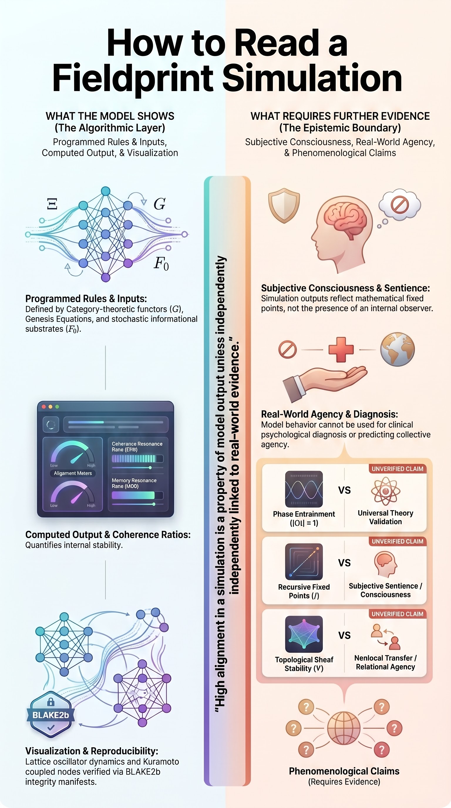
*Click image to expand.* Use the guide to identify the three regimes of coupled systems: incoherent spatial drift ($K < 1.0$), localized synchrony clustering ($1.0 \le K \le 3.0$), and global phase lock ($K > 3.0$).
Video Briefing: Decoding the Lattice
Listen to the principal theorists present the underlying Kuramoto coupling algorithms and explain what the simulator represents under epistemic conditions.
Duration: 6:00. This audio-visual walkthrough details the transition from discrete Cartesian observation neighborhoods to SHEAF-theoretic collective attunements.
Lattice Simulator Mechanical Blueprint & Epistemic Assumptions
To satisfy rigorous peer evaluation, this section maps the graphical user interface parameters of the Kuramoto coupled lattice simulation to its underlying mathematical formalism.
| UI Slider | Model Variable | Integration Range |
|---|---|---|
| Witness Intensity | Coupling $K$ | $[0.0, 10.0]$ |
| Coupling Radius | Adjacency $A_{ij}$ | $[30\text{px}, 120\text{px}]$ |
| Simulation Speed | Time Step $dt$ | $[0.02, 0.15]$ |
Adjusting *Witness Intensity* directly increases the coupling scalar $K$, forcing localized node synchronization. *Coupling Radius* alters the spatial metric threshold.
- Closed State Space: Intrinsic frequencies (\omega_i) are sampled from a uniform probability distribution \mathcal{U}(0.05, 0.10) and natural phases are bounded inside [0, 2\pi] radians.
- Phase Pull-In: Clicking nodes emits active phase-fronts that pull adjacent node phases (\theta_j) towards the target anchor (\theta_0) via a dampening ratio \theta_j \leftarrow 0.85 \theta_j + 0.15 \theta_0.
- Euler Forward Integration: Solved numerically via discrete Euler first-order forward steps, neglecting second-order torque/inertia.
Demonstrative Boundaries: This diagnostic tool runs a simplified local spatial coupled phase model. While useful for modeling collective behavior in mathematical physics, it has **zero empirical biological claims**.
This simulator is hosted strictly as a **pedagogical model illustration** of closed-system, self-referential phase locking. It does not establish clinical diagnoses, biological brainwave synchronization, or physical nonlocal state transfers.
Minimal Reference Implementation & Pseudocode
To satisfy academic reproducibility requirements, we provide clean, standalone, and mathematically exact implementations of the Kuramoto grid phase synchronization and order parameter () integration:
// Governing Kuramoto lattice update step
function stepKuramotoGrid(nodes, K, distThresh, dt) {
  const nextPhases = new Array(nodes.length);

  for (let i = 0; i < nodes.length; i++) {
    const nodeA = nodes[i];
    let couplingSum = 0;
    let neighborsCount = 0;

    for (let j = 0; j < nodes.length; j++) {
      if (i === j) continue;
      const nodeB = nodes[j];
      const dx = nodeB.x - nodeA.x;
      const dy = nodeB.y - nodeA.y;
      const distance = Math.hypot(dx, dy);

      if (distance < distThresh) {
        couplingSum += Math.sin(nodeB.phase - nodeA.phase);
        neighborsCount++;
      }
    }

    const couplingTerm = neighborsCount > 0
      ? (K * 0.1) / neighborsCount
      : 0;

    // First-order forward Euler integration
    nextPhases[i] = nodeA.phase + (nodeA.naturalFreq + couplingTerm * couplingSum) * dt;
    nextPhases[i] = (nextPhases[i] + Math.PI * 2) % (Math.PI * 2);
  }

  return nextPhases;
}import numpy as np
def calculate_coherence_index(phases):
"""
Computes the dimensionless Kuramoto order parameter (r).
phases: 1D array of phase angles in radians [0, 2*pi]
returns: r in [0.0, 1.0] where 1.0 is absolute phase lock.
"""
n = len(phases)
if n == 0:
return 0.0
# Convert phase angles to complex unit vectors
unit_vectors = np.exp(1j * np.array(phases))
# Calculate global average vector
average_vector = np.sum(unit_vectors) / n
# Absolute magnitude represents order parameter r
r = np.abs(average_vector)
return float(r)